
Contents of this article

In the previous article, we adjusted the weights of a portfolio with a fixed variance (risk). Continuing the topic of portfolio optimisation, in this article we approach portfolio optimisation through the efficient frontier.
What is the efficient frontier?
The efficient frontier (EF) is the curve representing the set of stock portfolios for which:
- The portfolio’s expected return is the highest for a fixed level of risk, or
- The portfolio’s risk is the lowest for a fixed level of expected return.
The efficient frontier is plotted as a scatter chart with two variables: return (y-axis), usually represented by the compound annual growth rate (CAGR), and risk (x-axis), usually represented by the portfolio’s variance.
So how is the efficient frontier determined, and why is it one of the tools that help us choose an efficient portfolio? Let’s move on to the next section.
Steps to build the efficient frontier
So far, we have only optimised a portfolio by choosing the one with the lowest risk (variance). We also know that for any given level of risk, there are always portfolios with different returns. In this section, we dig deeper into that idea, again with the aim of finding the optimal portfolio.
Going back to our familiar five-stock portfolio – VPB, HPG, VHM, VNM and FPT – the portfolio’s variance and expected return are 1.57% and 4.25% respectively. We will now raise the risk level to 2% and find the highest and lowest returns this portfolio can achieve.
Treating 1.57% as the lowest risk level, with a return of 4.25%, we will keep raising the portfolio’s risk and finding the highest and lowest returns, paying attention to the weights as well. After doing this, we will have a certain number of observations.
Finally, we plot these observations on a scatter chart (at each risk level, we have one data point for the highest return and one for the lowest; successive risk levels give us a set of data points that, when joined, form an arc-like curve).
Note that you are free to adjust the portfolio’s risk level for your own calculations; it depends entirely on your risk appetite. The 2% figure I use is just for the calculation, not a required number.
Step 1. Use the Solver tool
As explained in the previous article, when using the “Solver” tool to reach a desired target value (here, the expected return), we adjust other variables related to the target value. In this article, we adjust the weight of each stock in the portfolio so that its variance is as low as possible.
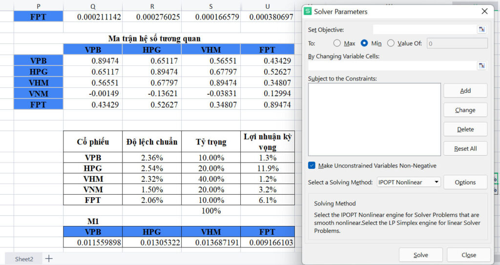
Step 2. Set the parameters
With risk fixed at 2%, we now need to find the portfolio’s highest return. The objective cell (the portfolio’s expected return) must therefore be set to “Max”, as follows:
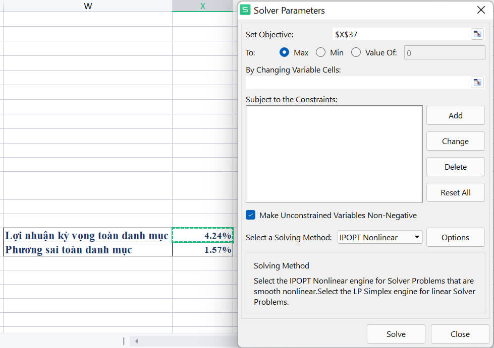
Step 3: Choose the weights to adjust
In this step, under “By Changing Variable Cells”, select the column of stock weights. The weights are the values that will change to maximise the portfolio’s expected return. Details below:

Step 4. Set the constraints
As in the previous article, in the “Subject to the Constraints” field we set the additional conditions beyond the two set above. Specifically, we need to ensure two other important conditions:
- The total weight of the portfolio must always equal 100%
- The portfolio’s total risk is fixed at 2%
As follows:

Click “Solve” to run it. The detailed result is as follows:
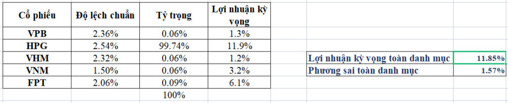
So with risk fixed at 2%, the portfolio’s maximum expected return is 11.85%. To achieve this, however, the weights have changed relative to those of the lowest-risk portfolio.
Having found the maximum expected return for a portfolio with 2% risk, we now need to find the minimum expected return. The steps are the same as before, except in step 2: instead of setting “Max”, this time we choose “Min”.

With all other conditions unchanged, the objective cell – the portfolio’s expected return – has gone from its maximum to its minimum, 1.22%. Clearly, with the same level of risk, we now have two separate stock portfolios with two different expected returns.
In summary, from one original portfolio we now have three portfolios:

Note that to draw the efficient frontier, we need many more portfolios (that is, more data points). So next, we calculate for many other risk levels to get more maximum and minimum expected returns and plot them on a scatter chart.
After the calculations, I have highlighted the two data columns needed for the chart (risk and expected return) to make it easier to follow.

After selecting the two data columns, click Insert and choose a scatter plot to visualise the data as the efficient frontier.

The chart above is a visual representation of the efficient frontier (EF). What does it tell us about portfolio optimisation, and why does it matter?
First, the leftmost point represents the portfolio with the lowest risk – our original portfolio (variance 1.57% and expected return 4.25%).
Second, apart from the leftmost point, at each level of risk (x-axis) there are always two corresponding points, a high return and a low return (y-axis). The higher point shows the high return our portfolio can achieve in favourable conditions, and the lower point the opposite.
Put simply, once we have determined the level of risk that suits our investment appetite, we should aim for the highest return (the upper point).
More broadly, as investors we should only target portfolios on the upper part of the curve (the upper line when we join the data points), because they represent the best, most efficient portfolios.
Happy Trading !
The “Stock Trading For A Living” Course
Green Chart designed this course to give students a solid foundation in fundamental analysis and stock valuation, and to show them how to integrate it effectively into their existing trading system, especially for traders who already use technical analysis. The programme includes five theory sessions and six months of hands-on trading practice in the real market with the lecturer.
See full course details here.