Portfolio Optimisation Methods (Part 1)

With any investment, what every investor wants is for their portfolio to achieve the highest possible return. In previous articles, we discussed the types of investment risk and how to identify them. Some types of risk can be spread out through portfolio diversification, while others cannot.

Overall, the ultimate goal of the measures we try to take is to maximise the portfolio’s return – in other words, to optimise our portfolio. 

In this article, we look at portfolio optimisation methods, starting with the most basic concepts.

What is portfolio optimisation?

Let’s start with a basic problem. Suppose you are considering two stocks, VPB and FPT, with expected returns of 22% and 15% respectively. You decide to split your capital equally between them (50:50). What will the expected return of the whole portfolio be?

It is very simple: we have each stock’s expected return and weight, so the portfolio return is calculated as follows:

= (Weight of VPB × Return of VPB) + (Weight of FPT × Return of FPT)

Applying the formula above, the result is:

50% × 22% + 50% × 15%

= 11% + 7.5%

= 18.5%

So the two-stock portfolio above is expected to return 18.5% a year.

If you don’t remember what a stock’s expected return is, you can reread our dedicated article on it here.

The next question is: does the expected return change when the weights change? What would the return be with a 30% / 70% split? 

There are two cases with that split:

Case 1: 30% VPB, 70% FPT:

Expected return = 30% × 22% + 70% × 15%

= 6.6% + 10.5%

= 17.1%

Case 2: 70% VPB, 30% FPT:

Expected return = 70% × 22% + 30% × 15%

= 15.4% + 4.5%

= 19.9%

We can clearly see that the expected return changes as the weights change. The example shows that the second case delivers a higher return. This leads to an important conclusion: a portfolio’s return and risk change when its weights change, because return is closely tied to risk.

Now extend this to a portfolio of n stocks: using historical data and analysing the different cases helps us determine which weights deliver the highest return. These steps are exactly what we do to optimise a portfolio. The aim of adjusting weights, or optimising a portfolio, is to:

• Find the weights that deliver the highest possible return, or
• Find the weights that minimise the portfolio’s risk.

Before going into the details of portfolio optimisation, let’s go through some important terms that will come up often in the sections ahead:

• Minimum-variance portfolio:  the portfolio whose weights give it the lowest risk. This type of portfolio is best suited to investors with a low risk appetite.
• Maximum-return portfolio: this type of portfolio has the weights that deliver the highest return, but its risk is correspondingly high. 
• Each fixed level of variance/risk corresponds to many portfolios: for each level of risk/variance, there can be at least two suitable portfolios. For example, with a variance/risk of 15%, there may be a portfolio returning 30%, while another may return only 12%. Note that the risk level is fixed but the return can vary. And between these two portfolios there are many others with different returns.

Steps to optimise a portfolio

In previous articles, we used a five-stock portfolio with the following weights:

The portfolio’s variance and expected return are 1.57% and 50.9% respectively. Our goal is to optimise this portfolio. In Excel, the Solver tool, found in the Data tab, is very useful for this.

Solver may not be enabled in Excel by default, in which case you need to install it under “Add-ins”. 

The steps we take to build a minimum-variance portfolio are:

Step 1: Lay out the data neatly and link the cells together, as follows:

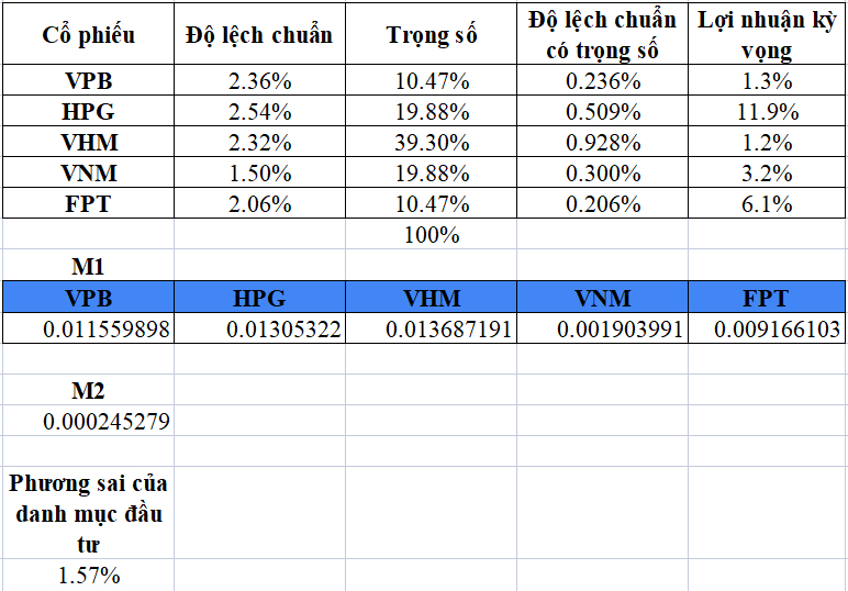
The part highlighted in blue is the most important: it is the input we use to optimise the portfolio. The data above it holds each stock’s weight, which will change as we optimise the portfolio.

Step 2: Use Excel’s “Solver” tool to optimise the portfolio. A few things to note about this tool: Solver helps solve problems where we need to find a “target value”, or a data point. The target is the result of a set of formulas that you can tune to reach a maximum, a minimum or a specified value, depending on your goal.

To do this, you adjust the values of certain input variables – the variables used in the formulas that produce the target value. In our problem, we use Solver to adjust the stock weights above so that the portfolio’s variance is as low as possible.

When you click Solver, a dialog box opens as shown above. Here we need to set the objective cell, which is the portfolio’s variance. The goal is to make this cell as small as possible (Min). 

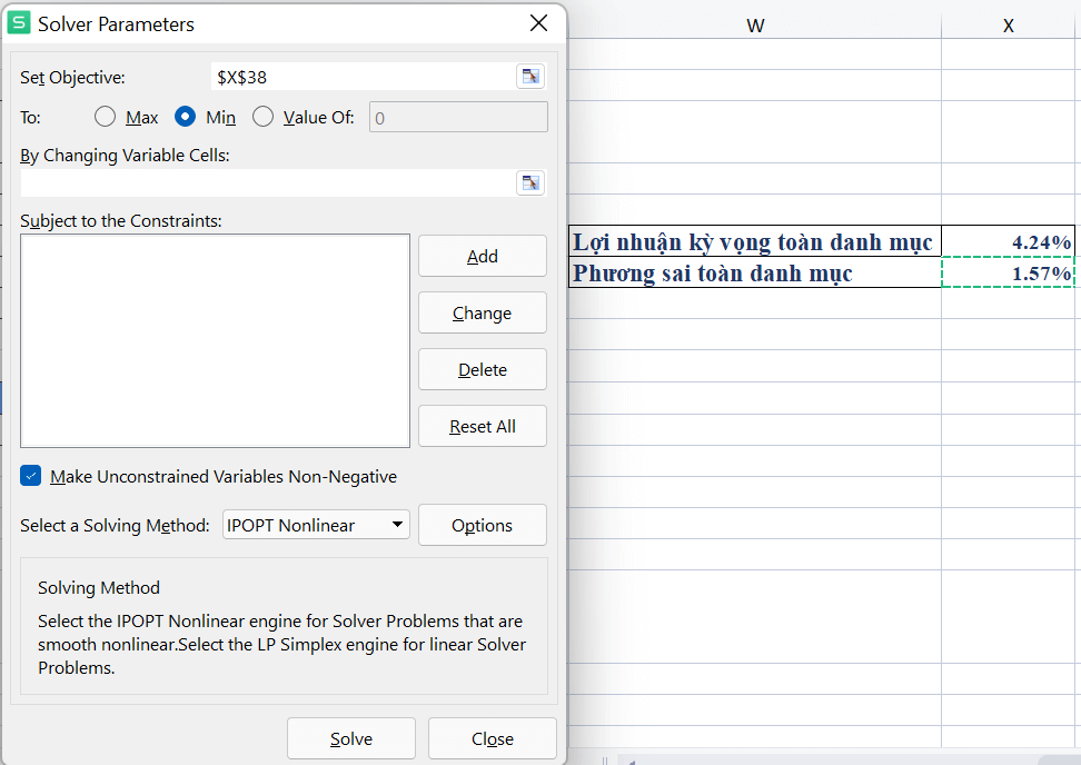
Next, we set the values Solver will change to minimise the objective cell. In our problem, the values that change are the weights of each stock.

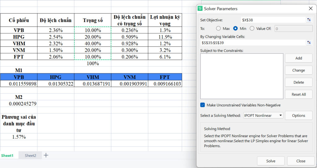
As you can see, in the “Changing Variable Cells” field I have selected the column of stock weights.

The dialog box also has a “Subject to the Constraints” field. This is where you specify whether, beyond the two requirements above, there are any other conditions to respect while adjusting the weights and optimising the portfolio. 

In our problem, one fixed condition is that the weights must always add up to 100%. To set this up, we do the following:

Click “Add”, and the following window appears:

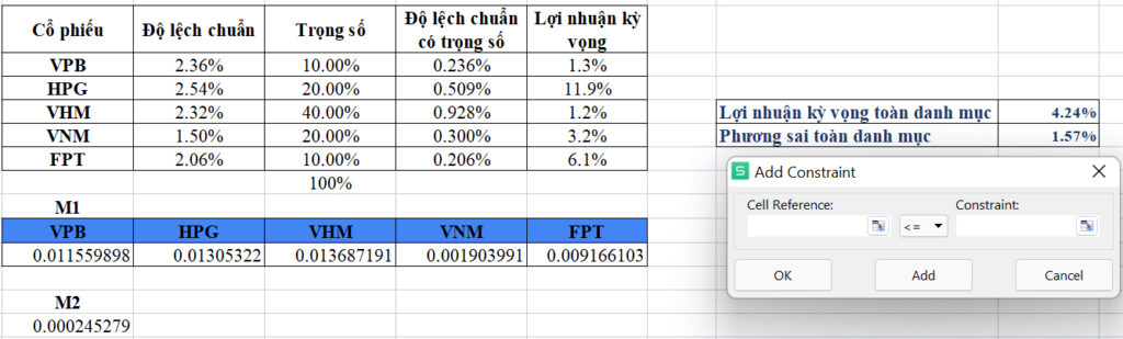
Set the constraint that the total weight must always equal 100%:

Watch the weights column, because after you click “Solve”, its values will change according to the conditions we set.

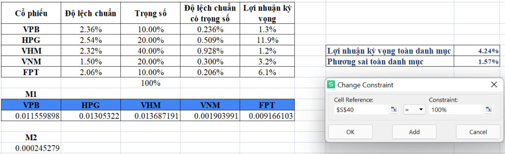
Watch the weights column, because after you click “Solve”, its values will change according to the conditions we set.

The weight of each stock has now changed. Although the change is small, remember that the dataset we are using covers only one month of trading. To see the reallocation clearly, apply the steps above to a dataset with more observations for a more complete picture!

Happy Trading !

The “Stock Trading For A Living” Course

Green Chart designed this course to give students a solid foundation in fundamental analysis and stock valuation, and to show them how to integrate it effectively into their existing trading system, especially for traders who already use technical analysis. The programme includes five theory sessions and six months of hands-on trading practice in the real market with the lecturer.

See full course details here.