
Contents of this article

When managing a portfolio, what we usually care about is the return of the portfolio as a whole. Instead of looking at numbers, there is a way to visualise portfolio returns as a picture that helps investors track them more easily: the equity curve.
What is the rate of return?
The return of a whole portfolio is the weighted average of the expected returns of each of its components. The weight of each component is its percentage of the portfolio’s total value.

What is the equity curve?
The equity curve is a line showing a portfolio’s return on a base of 100. Put more simply, it shows how $100 invested at the start would have performed over the observation period. With this measure, we can also easily compare the portfolio with major market indices such as the VN-Index or the VN30.
In this article, we build an equity curve for the five-stock portfolio from earlier examples to see how it performed over one month
Here is our portfolio, with the weight of each stock:
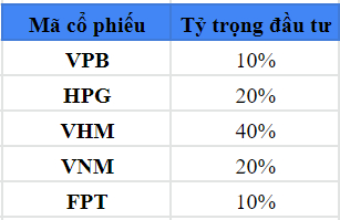
Note that the investment weight is the share of your total available capital that you allocate to each stock. In the example used in this article, with total capital of VND 10 million, we allocated VND 1 million to VPB, a 10% weight in the portfolio.

Next to the return column is the column with each stock’s weight. At the end of the row, we have the portfolio’s initial value (VND 10 million) and a total weight of 100%. Note that the weights of the five individual stocks must always add up to 100%.
Now let’s look at each stock in detail, starting with VPB. With a 10% weight, the initial investment in VPB is VND 1 million. From the change in closing price on 5 January compared with 4 January, we calculate the daily return and multiply it by 1 million. So the VND 1 million invested in VPB after 4 January becomes ~VND 985K. That is also the starting value to compare with the next day’s price.

On 4 January, we decide to buy VPB at VND 36.05K. In real trading, it is not easy to buy a stock at exactly the price you want and have it arrive in your account immediately (the T+2 rule).
In this example, however, we assume the trade is executed as soon as we decide. So on 4 January we use 10% of our money, VND 1 million, to buy VPB at VND 36.05K. The next day, VPB closes at VND 35.5K, down 1.53% from the previous day. This means the VND 1 million has fallen 1.53% to ~VND 985K.
Similarly, the next day VPB closes at VND 35.15K, so the investment falls 0.99% to ~VND 990K. For the following days, we apply the same logic to the rises and falls in the share price.
The image below illustrates the explanation above:

*The blue columns show the daily change in the money allocated to each stock.
The question here is: we initially allocated VND 10 million across five stocks with five different weights. But as share prices move each day, does the total of all the weighted values still equal VND 10 million?
Answering this question will show us how the portfolio moves.

As in the second row, calculating the total value for each day in turn gives us a time series of the portfolio’s value.

From that time series, we can plot the equity curve (EQ curve) as a line chart connecting the data points above. It looks like this:
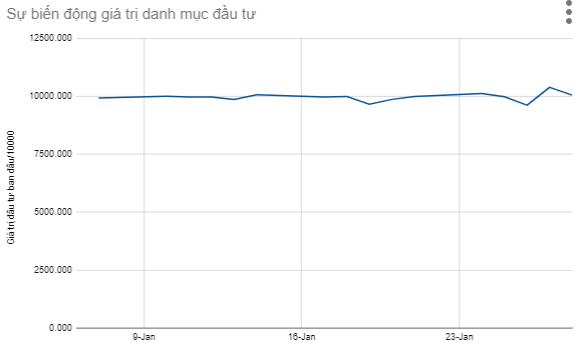
Very simple and visual, right? The equity curve is a very popular way to show a portfolio’s performance. It gives a quick estimate of the profit the portfolio has generated. In this case, we started with an investment of VND 10 million, and after one month the portfolio was valued at VND 10,043,564, as follows:

So, without much thought, we know the portfolio gained nearly 0.43% over the one-month observation period – which is also the portfolio’s return for the past month.
Another way to look at portfolio risk
In earlier articles, we learned how to calculate a portfolio’s variance from the standard deviations of the individual stocks. We also know that standard deviation represents a stock’s volatility, a measure of how risky the stock is.
To calculate standard deviation, we used Excel’s ‘=STDEV()’ function on the stock’s daily returns.
In this article, meanwhile, we have the portfolio’s daily value, fluctuating around the initial $1,000 invested. Imagine the portfolio is now just like a single stock: calculating its daily returns is the same as calculating a stock’s daily returns.
And if we apply ‘=STDEV()’ to the portfolio’s returns, are we not calculating its standard deviation – in other words, the risk/variance of the whole portfolio? Do you see the connection?
Exactly – we are calculating the portfolio’s variance with a completely new approach!
In the previous article, the portfolio variance we calculated was:
1.57%
We got that figure using matrix multiplication and the correlation matrix method.
In this article, we treat the portfolio as a single stock and calculate its daily returns. We then calculate the portfolio’s standard deviation from that return series. The final result is the same as the one we found above.
Here are the portfolio’s daily returns:

Once we have the daily return series, we use ‘=STDEV()’ to calculate the portfolio’s standard deviation.
As you can see, the result matches the figure we calculated in the previous article.
Happy Trading !
The “Stock Trading For A Living” Course
Green Chart designed this course to give students a solid foundation in fundamental analysis and stock valuation, and to show them how to integrate it effectively into their existing trading system, especially for traders who already use technical analysis. The programme includes five theory sessions and six months of hands-on trading practice in the real market with the lecturer.
See full course details here.