
Contents of this article

In investing, a common mindset is to forecast our returns in advance and expect them to be the largest figure we could receive in future. Taking a more objective view, however, we all have to admit that risk can sometimes arrive very suddenly and leave us little time to react.
That is why investors turn to risk-hedging measures to minimise potential losses. And to put these measures in place, estimating the maximum loss we are at risk of suffering is extremely important. In this article, we approach risk management through a very important concept: Value at Risk. First of all:
What is Value at Risk?
We have all heard the term “black swan“, popularised by Nassim Nicholas Taleb, which refers to extremely rare events that have had very serious consequences in history. Because they are so rare, black swan events defy all normal forecasts.
Why black swans, and what do they have to do with VaR?
The history of the world economy includes many “black swan” events with truly disastrous consequences. One is the dot-com bubble of 2001, when investors’ excessive expectations for dot-com companies (companies using the internet as the main platform for their business) led to sky-high valuations, even though these companies owned very few physical assets and had unclear profit histories.
When these companies reported profit shortfalls, investors quickly moved to other investments, triggering a sell-off that sent prices tumbling, and the collapse of many companies followed, with serious consequences for the economy.
Besides the dot-com bubble, an arguably even worse black swan event was the 2008 housing bubble, which started in the United States, crashed the US housing market and then spread around the world with very severe consequences.
In the same year, Zimbabwe fell into hyperinflation (the most severe form of inflation), with prices “jumping” hour by hour. At its peak, Zimbabwe’s inflation reportedly reached 500 billion percent, and the highest banknote was worth 100 trillion Zimbabwean dollars – issued just so that people would not have to cart wheelbarrows of cash to buy everyday necessities.

Hyperinflation in Zimbabwe
In situations like these, VaR becomes an effective tool for measuring the risk of investments and financial institutions (in this article, the risk of an investment portfolio), because it answers two important questions:
First, if a “black swan” event occurs, what is the largest loss our portfolio could suffer?
Second, what is the probability (%) of that happening?
To determine a portfolio’s VaR (not to be confused with variance, Var), the steps are as follows:
- Determine the distribution of the portfolio’s returns
- Build a frequency table to check whether the portfolio’s returns follow a normal distribution
- Sort the portfolio’s returns in descending order
- Select 95% of all observations
- The smallest value within that 95% of observations is the portfolio’s VaR
- The average of the last 5% of observations is called the CVaR (Conditional VaR)
When it comes to VaR, the foundational knowledge we need is the normal distribution, which we use to determine the distribution of the portfolio’s returns. Conveniently, we already calculated normalised returns in the article on the equity curve; you can review the steps here.
Once we have calculated the portfolio’s daily returns (1), we need to determine whether these returns follow a normal distribution (2). To do this, we go through a few basic steps:
Step 1: Find the portfolio’s minimum and maximum returns over the study period using the ‘=Max()’ and ‘=Min()’ functions in Excel.

Step 2 – Count the number of data points (observations) using the ‘=count()’ function

Our example portfolio has 126 return observations, matching the number of actual trading days in the dataset. Once you understand the steps in this example, you can apply them to a dataset with more observations (ideally one year or more) for the most complete and concrete view of the method.
Step 3 – Determine the interval between return levels (bin width)
The bin width is a fixed interval that divides the range of values into equal parts.
In this example, bin width = (difference between the maximum and minimum returns) / number of observations
= (3.26% – (-2.28%))/126
= 0.24%
Step 4 – Create the “bins_array”
To plot the portfolio’s returns as a distribution chart (histogram), we need two basic elements: the return and how often that return occurs. Since we have already calculated the return series, in this step we determine their frequency.
Frequency tells us how many times a particular return occurs – for example, “how many times did the portfolio return 0.5% over the past month?”. To determine frequency, we use Excel’s “=FREQUENCY” function, which has two required inputs:
- data_array: an array or reference to a set of values whose frequencies you want to count.
- bins_array: an array or reference to the intervals into which you want to group the values in data_array.
To build the bins_array, we successively add the bin width to each return level in the series. For example:
= -2.82% + 0.24%
= -2.58%
Doing the same for every return in the series gives us the following table:
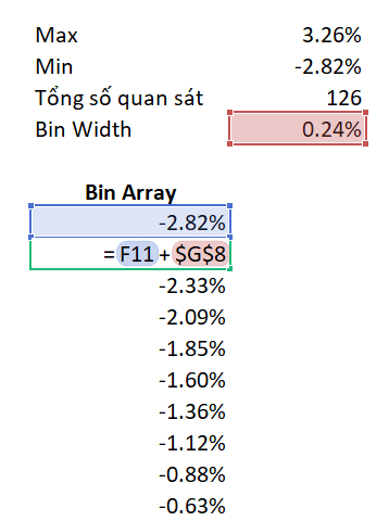
Next, we determine the frequency of the adjusted return levels we have just calculated using the ‘=frequency()’ function. The result is as follows:

Always remember that we are calculating over whole data arrays at once, so to run the function we need to press ‘Ctrl + Shift + Enter’ rather than just ‘Enter’.
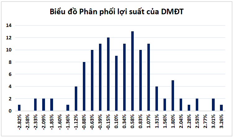
Step 5 – Plot the return distribution
Through the four steps above, we now have data on returns and their corresponding frequencies. At this step, we simply chart the frequencies to visualise their distribution. Once the chart is drawn, check whether the distribution looks like a bell curve (the characteristic shape of a normal distribution).
The result is as follows:
What is the portfolio’s Value at Risk?
Having established that the portfolio’s returns follow a normal distribution, we now determine the portfolio’s Value at Risk (VaR). First, sort the return series in descending order.

The portfolio’s VaR is defined as the smallest value within 95% of all observations. We have 126 observations in total, so 95% of them is about 120. In our example, VaR is therefore -1.48%.
For the remaining 5% of observations (6 observations), their average corresponds to the portfolio’s conditional VaR (CVaR). In our example, CVaR = -2.39%.
Some typical questions people ask when they first approach portfolio Value at Risk are:
Why do we need to check whether the portfolio’s returns follow a normal distribution?
When a dataset follows a normal distribution, about 68% of observations lie within one standard deviation (1 SD) of the mean, 95% within two standard deviations and 99.7% within three.
So when a portfolio’s returns are normally distributed, its return on any random day will fall within this 95% of observations. The smallest value within that 95% therefore represents the portfolio’s largest expected loss – the VaR.
With a VaR of -1.48%, could the portfolio lose even more?
The answer is that it certainly can, and that is what the portfolio’s CVaR captures. In exceptional cases, there is about a 5% chance that the portfolio’s loss exceeds the VaR, averaging -2.39% in the example above. The portfolio’s losses will rarely exceed this CVaR figure.
We hope that with what we have discussed above, you can apply these ideas to your own portfolio right away and gain deeper insight into it. VaR is an interesting way to gauge portfolio risk, and you can use it as a basis for adjusting your portfolio to suit your risk appetite.
Happy trading !
The “Stock Trading For A Living” Course
Green Chart designed this course to give students a solid foundation in fundamental analysis and stock valuation, and to show them how to integrate it effectively into their existing trading system, especially for traders who already use technical analysis. The programme includes five theory sessions and six months of hands-on trading practice in the real market with the lecturer.
See full course details here.