[TECHNICAL INSIGHTS] – The FFR and Its Impact on Market Regimes (Part 2)

Following on from Part 1, in this part we will use the variables observed so far to build a dashboard that tracks their movements and assesses their impact on the VN-Index.

Objectives of this post:

• Get a basic understanding of the FFR (Done).
• Briefly understand how the FedWatch Tool calculates probabilities and build a similar monitoring tool (Done).
• Understand the relationships between the variables and factors (Part 2).
• From these relationships, find regimes based on how this variable affects markets such as the S&P 500 and the VN-Index, to generate trade ideas (Part 3).

Conclusions of Part 2

Thanks for reading! Subscribe for free to receive new posts and support my work.

Looking further at the movements of other factors:

• Market indices: S&P 500, FTSE, DAX, Singapore, JP225
• Volatility measures: VIX, VVIX, VN-Index volatility, VN-Index breadth
• VN-Index fundamentals: P/E, P/B
• Changes in the FFR
• Changes in other alternative assets: gold, oil, BTC

we conclude that the variables affecting the VN-Index are (from strongest to weakest):

• The SPX and its movements (lags, means): very important, ranked first by weight.
• VVIX: the volatility of volatility, ranked second.
• Changes in oil prices.
• Movements in the Singapore market.
• Changes in the FFR, via log_distance.
• Movements in the German market.
• Past movements of the VN-Index and its fundamentals.
• Changes in gold and BTC.

Notes:

• This post is purely my personal view and analysis, based on my limited knowledge, so it is somewhat subjective. I would very much welcome everyone’s feedback!
• The writing style is close to everyday speech, not very academic, and sometimes mixes in English terms; I hope readers will bear with this.
• The data is accessed and calculated from the vnstocks library (http://vnstocks.com) and yfinance.
• Unlike some academic research, the goal here is to find influential factors to observe and forecast, so I keep speculation and conspiracy theories to a minimum – things like the VN-Index being moved by the SPX because of Trump, because of tariff policy, or “liquidity moves the market” (=]]), blah blah… Why?
  • Simply because I don’t want to fall into certain biases in financial reasoning, specifically anchoring bias (anchoring on limited knowledge) and confirmation bias (seeking information that confirms my argument and, intentionally or not, leaving out information pointing the other way).
  • The market is always changing; the information I have now explains only part of the movement, and often only from one angle. That means if we look at it differently, it may still be meaningful and can still be mined.
  • The goal here is not research either: I am looking for alpha, i.e. trading strategies. So signal testing matters more!

REGIMES

Analysing and assessing the impact

In Part 1, I looked at the FFR (Fed Funds Rate), the S&P 500 (SPX), gold prices (GOLD) and oil prices (OIL) to see their causal relationships with the VN-Index. This time it is similar, but extended with some more variables:

• Indices: FTSE (UK100), NK225 (Japan), Singapore_iShare (an ETF tracking the Singapore index), DAX (Germany), and the VIX and VVIX to measure S&P 500 volatility and the volatility of volatility (the VIX of the VIX);
• Other alternative assets: Bitcoin (BTC).

In addition, to limit the problem of non-stationary time series, I recalculated the “distance” variable from Part 1 (previously Market_FFR minus Current_FFR) as the difference between the logarithms of the two variables. This also reflects the continuous nature of interest rates. Testing all the variables for stationarity (ADF test), I get the following results:

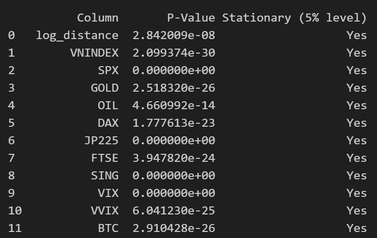
All the variables pass the stationarity test well. I then used these variables to compute a causality network, with Granger causality tests as the central measure and a 20-day return window, with the following result:

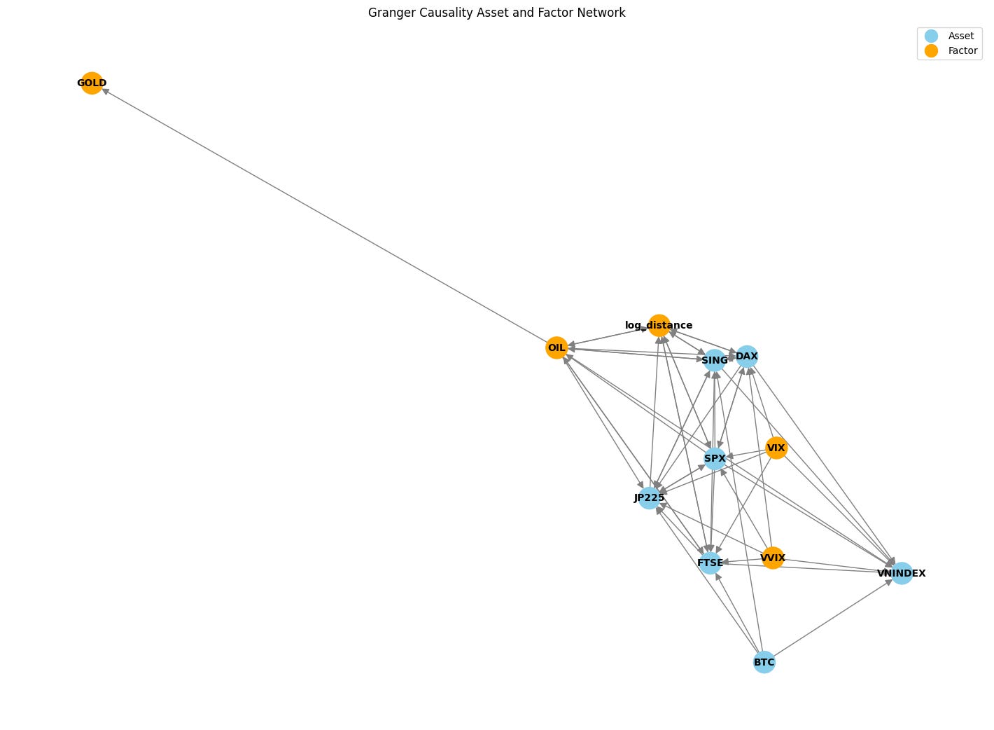
The result is quite a tangle (=.=) and not very clear, but with a magnifying glass I could make out a few findings:

• All the indices except JP225 directly affect the VN-Index (very interesting – I usually hear people say to watch JP225 =]]). All the relationships are one-way, with the influence running mainly towards the VN-Index.
• The only variable with a two-way causal relationship is oil (very interesting): it affects the VN-Index, and vice versa.
• Factor variables such as gold prices or changes in the FFR have no direct effect; instead, they work through some intermediate variable – gold through oil prices, and FFR changes through the FTSE, SPX, Singapore and DAX.
• And another interesting point: BTC directly affects the VN-Index (heh).

So based on historical data, with a 20-day window for returns and return lags, I found the results above. Normally, I would look at the charts of all these factors to assess their impact on the VN-Index and “guess” its near-term movement (e.g. over 20 days). But now a new question arises: how do we know which one matters most?

The Granger test only shows that a linear causal relationship exists between the pairs of variables above; it does not say how strongly each variable affects the VN-Index.

To solve this, I will use a measure called “elastic net” regression (sounds seriously scary =]]).

In the post analysing the impact of fundamental factors on the VN-Index, I listed some measures such as correlation and used some regression methods to limit multicollinearity. In this case, this regression method both removes the multicollinearity concern and identifies (linearly) how important each variable is to the target (the VN-Index).

So what is “elastic net” regression? Why does it work like this?

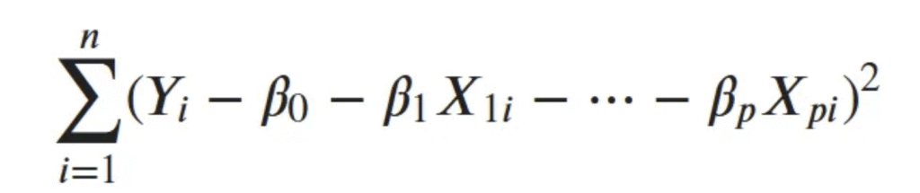
• Ordinary least squares (OLS) linear regression is very sensitive to outliers (values far from the observed range pull the regression line off its reasonable path) and to multicollinear variables. This means the OLS model fails at its main goal of minimising the residuals (it is no longer least squares). The model’s residual is calculated like this:

Statisticians have tackled this problem with several regression methods, including Ridge, Lasso and Elastic Net, as follows:

• These methods share a common approach: penalisation. What is penalisation? When you run the regression, you get the model’s parameters (Betas, or slopes), plus a component that penalises the Betas according to their influence (roughly, whoever talks nonsense or distorts things a lot gets punished). The function looks like this:

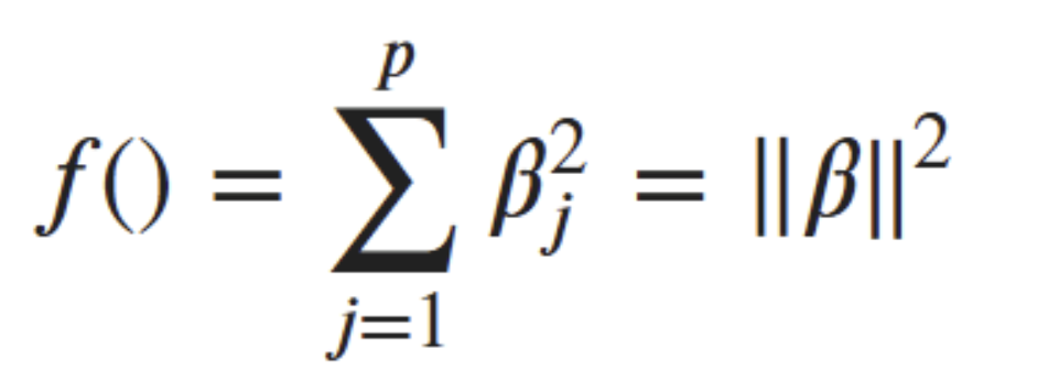
Ridge (L2): penalises with a function f(Beta) of this form:

• • That is, the sum of the squares of all the Betas (regardless of their signs). However, with too many features, this sum becomes very sensitive (it can be too large if the Betas are greater than 1, or too small if they are less than 1).
  • Ridge’s penalty function is called L2.
  • Ridge has a “merciful” trait: it keeps every feature and only penalises each one more or less heavily.
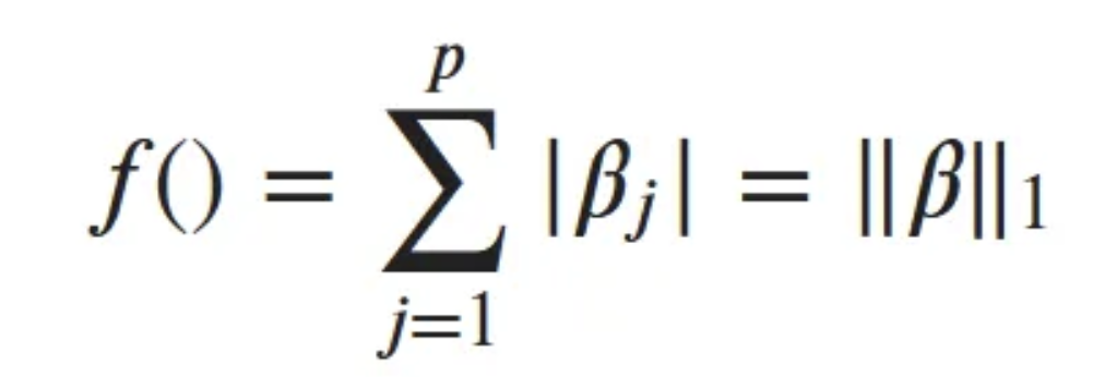
• Lasso (L1): solves this more thoroughly. Instead of squaring the Betas, Lasso takes their absolute values, like this:

• • This reduces the Betas’ sensitivity because they are not squared, so it can handle higher-dimensional data.
  • Lasso is more ruthless: it removes variables that are not meaningful to the model outright, thereby reducing the number of features (or dimensions).
• Elastic Net: combines the two above with L1 and L2 parameters, selecting a moderate number of variables while preserving explanatory power and limiting multicollinearity. The combination can be expressed by the following overall equation:

• • • You can see both Ridge’s and Lasso’s Beta penalties combined in the penalty equation above.

So I use Elastic Net and process the variables a little more, specifically:

• I add P/E and P/B variables to include fundamentals. These variables are “cooked” further with their standard deviation, moving average and z-score, as in the post analysing fundamental factors and the VN-Index.
• The variables above are cooked the same way, and I also add two lags of each variable.
• I also use the ADF test to check the stationarity of the variables before running the Elastic Net regression.
• The target variable is the VN-Index’s 1-day return. When running the regression, I use TimeseriesCV (mentioned in the fundamental-factors post) to find a suitable penalty constant for the equation and select suitable variables.
• After processing, there are 83 variables in total (@@).

In the end, I get the following results:

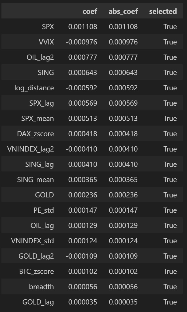
After one more round of filtering, the variables affecting the VN-Index are (from strongest to weakest):

• The SPX and its movements (lags, means): very important, ranked first by weight.
• VVIX: the volatility of volatility, ranked second.
• Changes in oil prices.
• Movements in the Singapore market.
• Changes in the FFR, via log_distance.
• Movements in the German market.
• Past movements of the VN-Index and its fundamentals.
• Changes in gold and BTC.

So based on these effects and the signs of the regression coefficients, I can build a dashboard from these indicators to get an overall view of their impact on the VN-Index. The weights follow each indicator’s importance, and the direction (up or down) follows the sign of the coefficient (coef in the table above). It looks like this:

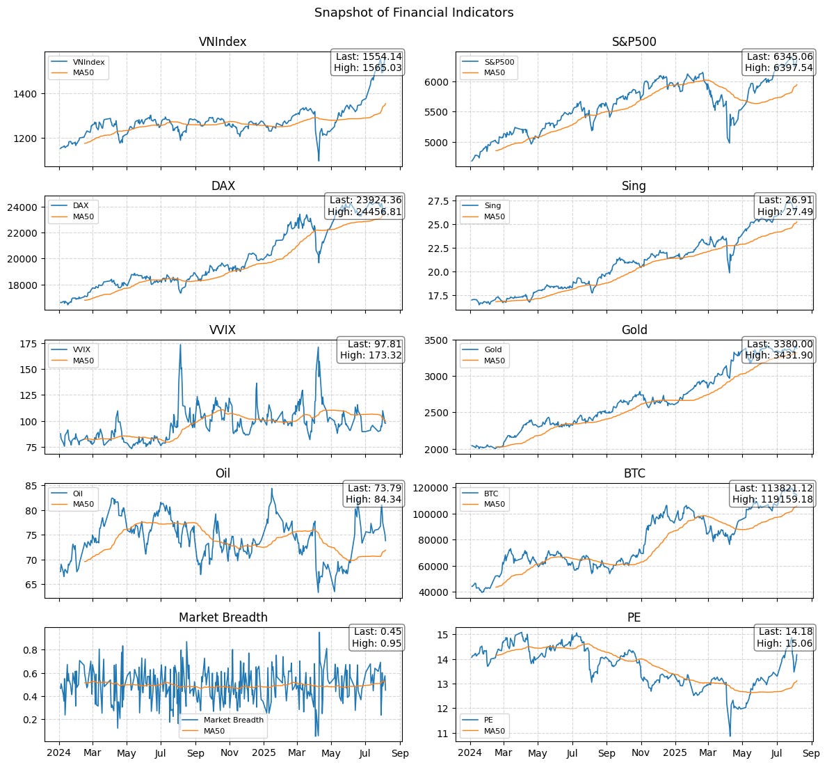
More ambitiously, though, I want to build a model to predict regimes from these indicators, for more stability than pure observation; I’ll save that for the next post.

That concludes this part; I hope it is useful to readers. Thank you!

Technical Analysis Course – CMT Level 1

Green Chart designed this course specifically for candidates in Vietnam who want to study and prepare for the CMT Level I exam. The programme includes 25 sessions of theory, practice questions and mock exams. Students also receive the course textbook, question bank and mock exams free of charge for their exam preparation, and can retake the course for free for life.

See more details about the course here.